Metrics
Introduction
Overview
metric signal
Before diving head first into the lab exercises, let’s start with a brief overview of OpenTelemetry’s metrics signal.
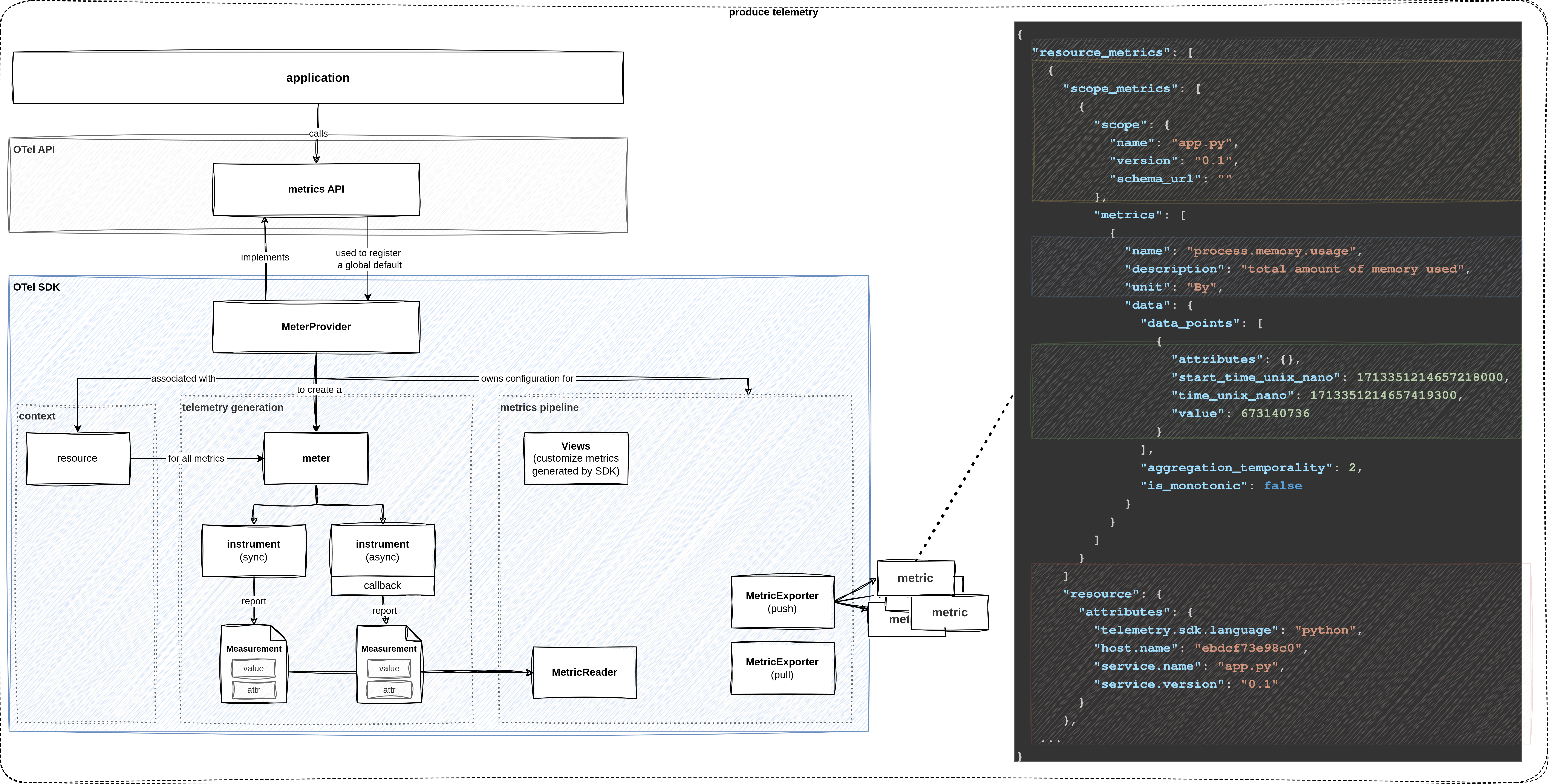
As usual, OpenTelemetry separates the API and the SDK.
The metrics API provides the interfaces that we use to instrument our application.
OpenTelemetry’s SDK ships with a official MeterProvider that implements the logic of the metrics signal.
To generate metrics, we first obtain a Meter which is used to create different types of instruments that report measurements.
After producing data, we must define a strategy for how metrics are sent downstream.
A MetricReader collects the measurements of associated instruments.
The paired MetricExporter is responsible for getting the data to the destination.
Learning Objectives
By the end of this lab, you will be able to:
- use the OpenTelemetry API and configure the SDK to generate metrics
- understand the basic structure and dimensions of a metric
- create and record measurements with the help of different types of instruments
- customize metrics are collected by the SDK
How to perform the exercises
This lab excercise demonstrates how to collect metrics from a Python application. The purpose of the exercises is to learn about OpenTelemetry’s metrics signal. It does not provide a realistic deployment scenario. In production, we typically collect, store and query metrics in a dedicated backend such as Prometheus. Prometheus uses a pull-based approach. Metrics are exposed as an HTTP endpoint and Prometheus server discovers and scrapes these target at regular intervals. In this lab, we output metrics to the local console to keep things simple. The environment consists of a Python service that we want to instrument. It is built with the Flask web framework, listens on port 5000 and serves serveral HTTP endpoints.
- This exercise is based on the following repository repository
- All exercises are in the subdirectory
exercises. There is also an environment variable$EXERCISESpointing to this directory. All directories given are relative to this one. - Initial directory:
manual-instrumentation-metrics/initial - Solution directory:
manual-instrumentation-metrics/solution - Python source code:
manual-instrumentation-metrics/initial/srcThe environment consists of two components:
- a Python service
- uses Flask web framework
- listens on port 5000 and serves serveral HTTP endpoints
- simulates an application we want to instrument
- echo server
- listens on port 6000, receives requests and sends them back to the client
- called by the Python application to simulate communication with a remote service
- allows us to inspect outbound requests
To work on this lab, open three terminals.
- Terminal to run the echo server
Navigate to
cd $EXERCISES
cd manual-instrumentation-metrics/initial
Start the echo server using
docker compose up- Terminal to run the application and view it’s output
Change to the Python source directory
cd $EXERCISES
cd manual-instrumentation-metrics/initial/src
Start the Python app/webserver
python app.py- Terminal to send request to the HTTP endpoints of the service
The directory doesn’t matter here
Test the Python app:
curl -XGET localhost:5000; echoTo keep things concise, code snippets only contain what’s relevant to that step.
If you get stuck, you can find the solution in the exercises/manual-instrumentation-metrics/solution
Configure metrics pipeline and obtain a meter
Let’s create a new file metric_utils.py inside the src directory.
We’ll use it to bundle configuration related to the metrics signal.
At the top of the file, specify the following imports for OpenTelemetry’s metrics SDK.
Then, create a new function create_metrics_pipeline.
In a production scenario, one would deploy a backend to store and a front-end to analyze time-series data.
Create a ConsoleMetricExporter to write a JSON representation of metrics generated by the SDK to stdout.
Next, we instantiate a PeriodicExportingMetricReader that collects metrics at regular intervals and passes them to the exporter. Add the following code to the file metric_utils.py.
# OTel SDK
from opentelemetry.sdk.metrics.export import (
    ConsoleMetricExporter,
    PeriodicExportingMetricReader,
    MetricReader,
)

def create_metrics_pipeline(export_interval: int) -> MetricReader:
    console_exporter = ConsoleMetricExporter()
    reader = PeriodicExportingMetricReader(
        exporter=console_exporter, export_interval_millis=export_interval
    )
    return reader
Then, define a new function create_meter.
To obtain a Meter we must first create a MeterProvider.
To connect the MeterProvider to our metrics pipeline, pass the PeriodicExportingMetricReader to the constructor.
As before with Traces, we will connect resource attributes with the MeterProvider, so they will be written into metric signals as well.
Use the metrics API to register the global MeterProvider and retrieve the meter. Extend the file with the following code:
# OTel API
from opentelemetry import metrics as metric_api

# OTel SDK
from opentelemetry.sdk.metrics import MeterProvider

# Resource Util
from resource_utils import create_resource

def create_meter(name: str, version: str) -> metric_api.Meter:
    # configure provider
    metric_reader = create_metrics_pipeline(5000)
    rc = create_resource(name, version)
    provider = MeterProvider(
        metric_readers=[metric_reader],
        resource=rc
    )

    # obtain meter
    metric_api.set_meter_provider(provider)
    meter = metric_api.get_meter(name, version)
    return meter
Finally, open app.py and import create_meter.
Invoke the function and assign the return value to a global variable meter.
# custom
from metric_utils import create_meter

# global variables
app = Flask(__name__)
meter = create_meter("app.py", "0.1")
Create instruments to record measurements
As you have noticed, thus far, everything was fairly similar to the tracing lab.
However, in contrast to tracers, we do not use meters directly to generate metrics.
Instead, meters produce (and are associated with) a set of instruments.
An instrument reports measurements, which represent a data point reflecting the state of a metric at a particular point in time. So a meter can be seen as a factory for creating instruments and is associated with a specific library or module in your application. Instruments are the objects that you use to record metrics and represent specific metric types, such as counters, gauges, or histograms. Each instrument has a unique name and is associated with a specific meter. Measurements are the individual data points that instruments record, representing the current state of a metric at a specific moment in time. Data points are the aggregated values of measurements over a period of time, used to analyze the behavior of a metric over time, such as identifying trends or anomalies.
To illustrate this, consider a scenario where you want to measure the number of requests to a web server. You would use a meter to create an instrument, such as a counter, which is designed to track the number of occurrences of an event. Each time a request is made to the server, the counter instrument records a measurement, which is a single data point indicating that a request has occurred. Over time, these measurements are aggregated into data points, which provide a summary of the metric’s behavior, such as the total number of requests received.
overview of different instruments
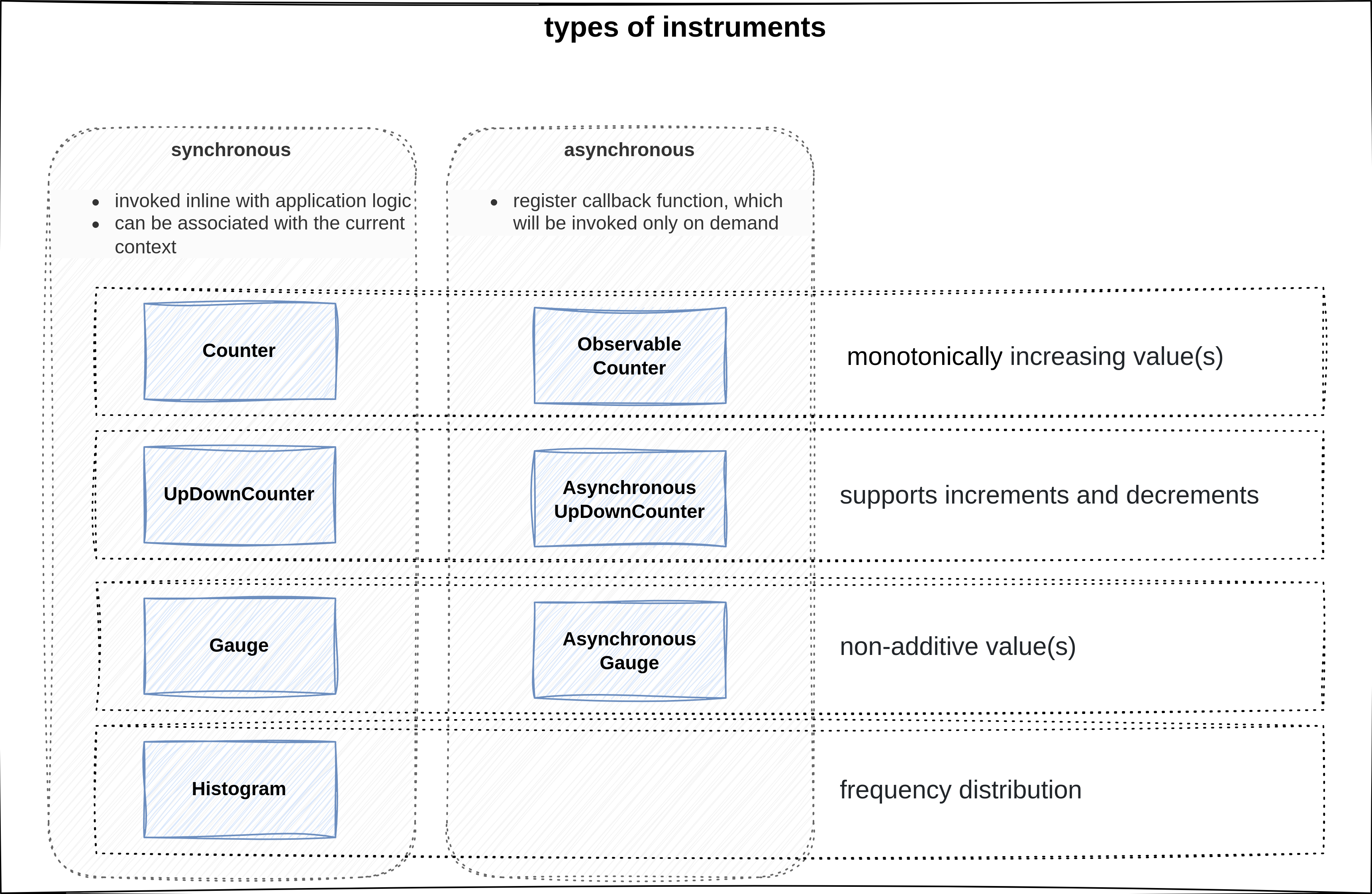
Similar to the real world, there are different types of instruments depending on what you try to measure. OpenTelemetry provides different types of instruments to measure various aspects of your application. For example:
Countersare used for monotonically increasing values, such as the total number of requests handled by a server.UpAndDownCountersare used to track values that can both increase and decrease, like the number of active connections to a databaseGaugeinstruments reflect the state of a value at a given time, such as the current memory usage of a process.Histograminstruments are used to analyze the distribution of how frequently a value occurs, which can help identify trends or anomalies in the data.
Each type of instrument, except for histograms, has a synchronous and asynchronous variant. Synchronous instruments are invoked in line with the application code, while asynchronous instruments register a callback function that is invoked on demand. This allows for more efficient and flexible metric collection, especially in scenarios where the metric value is expensive to compute or when the metric value changes infrequently.
For now, we will focus on the basic concepts and keep things simple, but as you become more familiar with OpenTelemetry, you will be able to leverage these components to create more sophisticated metric collection and analysis strategies.
In metric_utils.py add a new function create_request_instruments.
Here, we’ll define workload-related instruments for the application.
As a first example, use the meter to create a Counter instrument to measure the number of requests to the / endpoint.
Every instrument must have a name, but we’ll also supply the unit of measurement and a short description.
def create_request_instruments(meter: metric_api.Meter) -> dict[str, metric_api.Instrument]:
    index_counter = meter.create_counter(
        name="index_called",
        unit="request",
        description="Total amount of requests to /"
    )

    instruments = {
        "index_counter": index_counter,
    }
    return instruments
For analysis tools to interpret the metric correctly, the name should follow OpenTelemetry’s semantic conventions and the unit should follow the Unified Code for Units of Measure (UCUM).
Now that we have defined our first instrument, import the helper function into app.py.
Let’s generate some metrics.
Call create_request_instruments in the file’s main section and assign it to a global variable.
In our index function, reference the counter instrument and call the add method to increment its value.
from metric_utils import create_meter, create_request_instruments

@app.route("/", methods=["GET", "POST"])
def index():
    request_instruments['index_counter'].add(1)
    # ...

if __name__ == "__main__":
    request_instruments = create_request_instruments(meter)
    # ...
Start the web server using
python app.pyUse the second terminal to send a request to / via
curl -XGET localhost:5000; echoObserve the result in the terminal window where the python app is executed:
"resource": { // <- origin
    "attributes": {
        "telemetry.sdk.language": "python",
        "telemetry.sdk.name": "opentelemetry",
        "telemetry.sdk.version": "1.24.0",
        "service.name": "unknown_service"
    },
},
"scope_metrics": [
    {
        "scope": { // <-- defined by meter
            "name": "app.py",
            "version": "0.1",
            "schema_url": ""
        },
        "metrics": [
            {
                "name": "index_called", // <-- identify instrument
                "description": "Total amount of requests to /",
                "unit": "request",
                "data": {
                    "data_points": [ // <-- reported measurements
                        {
                            "attributes": {},
                            "start_time_unix_nano": 1705676073229533664,
                            "time_unix_nano": 1705676101944590149,
                            "value": 1
                        }
                    ],
                    "aggregation_temporality": 2, // <-- aggregation
                    "is_monotonic": true
                }
            }
        ],
    }
]
The scope_metrics array contains metrics scopes, each representing a logical unit of the application code with which the telemetry is associated. Each scope includes a scope section that identifies the instrumentation scope, such as the name and version of the instrumented module or library, and an optional schema URL. The metrics array within each scope contains the actual metrics reported by instruments associated with the meter, with each metric having a name, description, unit, and data points. The data points include attributes, timestamps, and the value of the measurement, along with properties that describe the aggregation temporality and whether the metric is monotonic.
The PeriodicExportingMetricReader records the state of metrics from the SDK at a regular interval and ConsoleMetricExporter writes a JSON representation to stdout.
Similar to tracing, we can attach a resource to the telemetry generated by the MeterProvider.
The JSON snippet provided is an example of the OpenTelemetry metrics data model, which is a structured representation of telemetry data collected from an application.
The resource section describes the entity being monitored, such as a service or a host, and includes attributes like the language of the telemetry SDK, the SDK’s name and version, and the service’s name.
The scope_metrics section has two main parts.
First, the instrumentation scope identifies a logical unit in the application code with which the telemetry is associated.
It represents the name and version parameters we passed to get_meter.
The metrics field contains a list of metrics reported by instruments associated with the meter.
Each metric consists of two main parts.
First, there is information to identify the instrument (e.g. name, kind, unit, and description).
Second, the data contains a list of data_points, which are measurements recorded by the instrument.
Each measurement typically consists of a value, attributes, and a timestamp.
The aggregation_temporality indicates whether the metric is cumulative, and is_monotonic specifies whether the metric only increases (or decreases, in the case of a gauge). This model is designed to be flexible and extensible, ensuring compatibility with existing monitoring systems and standards like Prometheus and StatsD, facilitating interoperability with various monitoring tools.
Metric dimensions
So far, we only used the add method to increment the counter.
However, add also has a second optional parameter to specify attributes.
This brings us to the topic of metric dimensions.
To illustrate their use, modify the index function as shown below.
from flask import Flask, make_response, request

@app.route("/", methods=["GET", "POST"])
def index():
    request_instruments["index_counter"].add(
        1,
        { "http.request.method": request.method }
    )
Send a couple of POST and GET requests to / via
curl -XPOST localhost:5000; echocurl -XGET localhost:5000; echoLook at the output, what do you notice?
"data_points": [
    {
        "attributes": {
            "http.request.method": "POST"
        },
        "start_time_unix_nano": 1705916954721405005,
        "time_unix_nano": 1705916975733088638,
        "value": 1
    },
    {
        "attributes": {
            "http.request.method": "GET"
        },
        "start_time_unix_nano": 1705916954721405005,
        "time_unix_nano": 1705916975733088638,
        "value": 1
    }
],
We can conclude that the instrument reports separate counters for each unique combination of attributes. This can be incredibly useful. For example, if we pass the status code of a request as an attribute, we can track distinct counters for successes and errors. While it is tempting to be more specific, we have to be careful with introducing new metric dimensions. The number of attributes and the range of values can quickly lead to many unique combinations. High cardinality means we have to keep track of numerous distinct time series, which leads to increased storage requirements, network traffic, and processing overhead. Moreover, specific metrics may have less aggregative quality, which can make it harder to derive meaningful insights.
In conclusion, the selection of metric dimensions is a delicate balancing act. Metrics with high cardinality can lead to numerous unique combinations. They result from introducing many attributes or a wide range of values, like IDs or error messages. This can increase storage requirements, network traffic, and processing overhead, as each unique combination of attributes represents a distinct time series that must be tracked. Moreover, metrics with low aggregative quality may be less useful when aggregated, making it more challenging to derive meaningful insights from the data. Therefore, it is essential to carefully consider the dimensions of the metrics to ensure that they are both informative and manageable within the constraints of the monitoring system.
Instruments to measure golden signals
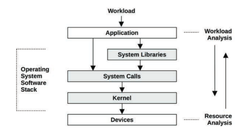
workload and resource analysis
Now, let’s put our understanding of the metrics signal to use. Before we do that, we must address an important question: What do we measure? Unfortunately, the answer is anything but simple. Due to the vast amount of events within a system and many statistical measures to calculate, there are nearly infinite things to measure. A catch-all approach is cost-prohibitive from a computation and storage point, increases the noise which makes it harder to find important signals, leads to alert fatigue, and so on. The term metric refers to a statistic that we consciously chose to collect because we deem it to be important. Important is a deliberately vague term, because it means different things to different people. A system administrator typically approaches an investigation by looking at the utilization or saturation of physical system resources. A developer is usually more interested in how the application responds, looking at the applied workload, response times, error rates, etc. In contrast, a customer-centric role might look at more high-level indicators related to contractual obligations (e.g. as defined by an SLA), business outcomes, and so on. The details of different monitoring perspectives and methodologies (such as USE and RED) are beyond the scope of this lab. However, the four golden signals of observability often provide a good starting point:
- Traffic: volume of requests handled by the system
- Errors: rate of failed requests
- Latency: the amount of time it takes to serve a request
- Saturation: how much of a resource is being consumed at a given time
Let’s instrument our application accordingly.
Traffic
Let’s measure the total amount of traffic for a service.
First, go to create_request_instruments and index to delete everything related to the index_counter instrument.
Incrementing a counter on every route we serve would lead to a lot of code duplication.
Modify the 2 source files to look like this:
def create_request_instruments(meter: metric_api.Meter) -> dict:
    traffic_volume = meter.create_counter(
        name="traffic_volume",
        unit="request",
        description="total volume of requests to an endpoint",
    )

    instruments = {
        "traffic_volume": traffic_volume,
    }

return instruments@app.route("/", methods=["GET", "POST"])
def index():
do_stuff()
current_time = time.strftime("%a, %d %b %Y %H:%M:%S", time.gmtime())
return f"Hello, World! It's currently {current_time}"Instead, let’s create a custom function before_request_func and annotate it with Flask’s @app.before_request decorator.
Thereby, the function is executed on incoming requests before they are handled by the view serving a route.
@app.before_request
def before_request_func():
    request_instruments["traffic_volume"].add(
        1, attributes={"http.route": request.path}
    )
Send a couple of POST and GET requests to / via
curl -XPOST localhost:5000; echocurl -XGET localhost:5000; echoLook at the output. Do you see the difference?
Error rate
As a next step, let’s track the error rate of the service. Create a separate Counter instrument. Ultimately, the decision of what constitutes a failed request is up to us. In this example, we’ll simply refer to the status code of the response.
Add error_rate to metric_utils.py as described here:
def create_request_instruments(meter: metric_api.Meter) -> dict:
   # ...
   error_rate = meter.create_counter(
        name="error_rate",
        unit="request",
        description="rate of failed requests"
    )

    instruments = {
        "traffic_volume": traffic_volume,
        "error_rate": error_rate,
    }
To access it, create a function after_request_func and use Flask’s @app.after_request decorator to execute it after a view function returns.
Modify the code according to this snippet:
from flask import Flask, make_response, request, Response

@app.after_request
def after_request_func(response: Response) -> Response:
    if response.status_code >= 400:
        request_instruments["error_rate"].add(1, {
                "http.route": request.path,
                "http.response.status_code": response.status_code
            }
        )
    return response
Latency
The time it takes a service to process a request is a crucial indicator of potential problems. The tracing lab showed that spans contain timestamps that measure the duration of an operation. Traces allow us to analyze latency in a specific transaction. However, in practice, we often want to monitor the overall latency for a given service. While it is possible to compute this from span metadata, converting between telemetry signals is not very practical. For example, since capturing traces for every request is resource-intensive, we might want to use sampling to reduce overhead. Depending on the strategy, sampling may increase the probability that outlier events are missed. Therefore, we typically analyze the latency via a Histogram. Histograms are ideal for this because they represent a frequency distribution across many requests. They allow us to divide a set of data points into percentage-based segments, commonly known as percentiles. For example, the 95th percentile latency (P95) represents the value below which 95% of response times fall. A significant gap between P50 and higher percentiles suggests that a small percentage of requests experience longer delays. A major challenge is that there is no unified definition of how to measure latency. We could measure the time a service spends processing application code, the time it takes to get a response from a remote service, and so on. To interpret measurements correctly, it is vital to have information on what was measured.
Let’s use the meter to create a Histogram instrument.
Refer to the semantic conventions for HTTP Metrics for an instrument name and preferred unit of measurement.
To measure the time it took to serve the request, we’ll use our before_request_func and after_request_func functions.
In before_request_func, create a timestamp for the start of the request and add it to the request context.
In after_request_func, take a timestamp for the end of the request and subtract them to calculate the duration.
We often need additional context to draw the right conclusions.
For example, a service’s latency number might indicate fast replies.
Add request_latency to metric_utils.py as described here:
def create_request_instruments(meter: metric_api.Meter) -> dict:
   # ...
   request_latency = meter.create_histogram(
        name="http.server.request.duration",
        unit="s",
        description="latency for a request to be served",
    )

    instruments = {
        "traffic_volume": traffic_volume,
        "error_rate": error_rate,
        "request_latency": request_latency,
    }
However, in reality, the service might be fast because it serves errors instead of replies.
Therefore, let’s add some additional attributes. Modify the code according to this snippet:
@app.before_request
def before_request_func():
   # ...
   request.environ["request_start"] = time.time_ns()

@app.after_request
def after_request_func(response: Response) -> Response:
    # ...
    request_end = time.time_ns()
    duration = (request_end - request.environ["request_start"]) / 1_000_000_000 # convert ns to s
    request_instruments["request_latency"].record(
        duration,
        attributes = {
            "http.request.method": request.method,
            "http.route": request.path,
            "http.response.status_code": response.status_code
        }
    )
    return response
To test if everything works, run the app, use curl to send a request, and locate the Histogram instrument in the output.
Before you do that stop the app Ctrl+C and start it with some filtered output:
python app.py | tail -n +3 | jq '.resource_metrics[].scope_metrics[].metrics[] | select (.name=="http.server.request.duration")'curl -XPOST localhost:5000; echocurl -XGET localhost:5000; echoYou should see that the request was associated with a bucket. Note that conventions recommend seconds as the unit of measurement for the request duration.
{
"name": "http.server.request.duration",
"description": "latency for a request to be served",
"unit": "s",
"data": {
    "data_points": [
        {
            "attributes": {
                "http.request.method": "POST",
                "http.route": "/",
                "http.response.status_code": 200
            },
            "start_time_unix_nano": 1705931460176920755,
            "time_unix_nano": 1705931462026489226,
            "count": 1,
            "sum": 0.107024987,
            "bucket_counts": [0,1,0,0,0,0,0,0,0,0,0,0,0,0,0,0], // <- frequency
            "explicit_bounds": [ 0.0, 5.0, 10.0, 25.0, 50.0, 75.0, 100.0, 250.0, 500.0, 750.0, 1000.0, 2500.0, 5000.0, 7500.0, 10000.0 ], // <- buckets
            "min": 0.107024987,
            "max": 0.107024987
        }
    ],
    "aggregation_temporality": 2
}
We expect a majority of requests to be served in milliseconds. Therefore, the default bucket bounds defined by the Histogram aren’t a good fit. We’ll address this later, so ignore this for now.
Saturation
All the previous metrics have been request-oriented. For completeness, we’ll also capture some resource-oriented metrics. According to Google’s SRE book, the fourth golden signal is called “saturation”. Unfortunately, the terminology is not well-defined. Brendan Gregg, a renowned expert in the field, defines saturation as the amount of work that a resource is unable to service. In other words, saturation is a backlog of unprocessed work. An example of a saturation metric would be the length of a queue. In contrast, utilization refers to the average time that a resource was busy servicing work. We usually measure utilization as a percentage over time. For example, 100% utilization means no more work can be accepted. If we go strictly by definition, both terms refer to separate concepts. One can lead to the other, but it doesn’t have to. It would be perfectly possible for a resource to experience high utilization without any saturation. However, Google’s definition of saturation, confusingly, resembles utilization. Let’s put the matter of terminology aside.
Let’s measure some resource utilization metrics.
To keep things simple, we already installed the psutil library for you.
Create a function create_resource_instruments to obtain instruments related to resources.
Use the meter to create an ObservableGauge to track the current CPU utilization and an ObservableUpDownCounter to record the memory usage.
Since both are asynchronous instruments, we also define two callback functions that are called on demand and return an Observation.
import psutil

# callbacks for asynchronous instruments
def get_cpu_utilization(opt: metric_api.CallbackOptions) -> metric_api.Observation:
    cpu_util = psutil.cpu_percent(interval=None) / 100
    yield metric_api.Observation(cpu_util)

def create_resource_instruments(meter: metric_api.Meter) -> dict:
    cpu_util_gauge = meter.create_observable_gauge(
        name="process.cpu.utilization",
        callbacks=[get_cpu_utilization],
        unit="1",
        description="CPU utilization since last call",
    )

    instruments = {
        "cpu_utilization": cpu_util_gauge
    }
    return instruments
Open app.py, import create_resource_instruments, and call it inside the main section.
With our golden signals in place, let’s use load-testing tools to simulate a workload.
import logging
from metric_utils import create_meter, create_request_instruments, create_resource_instruments

if __name__ == "__main__":
    # disable logs of builtin webserver for load test
    logging.getLogger("werkzeug").disabled = True

    # instrumentation
    request_instruments = create_request_instruments(meter)
    create_resource_instruments(meter)

    # launch app
    db = ChaosClient(client=FakerClient())
    app.run(host="0.0.0.0", debug=True)
We’ll use ApacheBench, which is a single-threaded CLI tool for benchmarking HTTP web servers.
Flask’s app.run() starts a built-in web server that is meant for development purposes.
Running a stress test and logging requests would render the console useless.
To observe the output of the ConsoleMetricExporter, add a statement to disable the logger.
Start the app and filter the output
# start app and filter output
python app.py | tail -n +3 | jq '.resource_metrics[].scope_metrics[].metrics[] | select (.name=="process.cpu.utilization")'
Run the ab command to apply the load, and examine the metrics rendered to the terminal.
# apache bench
ab -n 50000 -c 100 http://localhost:5000/users
Views
So far, we have seen how to generate some metrics. Views let us customize how metrics are collected and output by the SDK.
Before we begin, create a new function create_views.
To register views, we pass them to the MeterProvider.
The definition of a View consists of two parts.
First, we must match the instrument(s) that we want to modify.
The View constructor provides many criteria to specify a selection.
from opentelemetry.sdk.metrics.view import (
    View,
    DropAggregation,
    ExplicitBucketHistogramAggregation,
)

def create_views() -> list[View]:
    views = []
    return views

def create_meter(name: str, version: str) -> metric_api.Meter:
    metric_reader = create_metrics_pipeline(5000)
    rc = create_resource(name, version)
    views = create_views()

    provider = MeterProvider(
        metric_readers=[metric_reader],
        resource=rc,
        views=views # <-- register views
    )
Nothing prevents us from defining Views that apply to multiple instruments. Second, we must instruct the View on how to modify the metrics stream. Let’s look at some examples to illustrate why Views can be useful.
Modify the code as shown below:
# import instrument types
from opentelemetry.metrics import Histogram

def create_views() -> list[View]:
   views = []
   # adjust aggregation of an instrument
   histrogram_explicit_buckets = View(
      instrument_type=Histogram,
      instrument_name="*",  #  wildcard pattern matching
      aggregation=ExplicitBucketHistogramAggregation((0.005, 0.01, 0.025, 0.05, 0.075, 0.1, 0.25, 0.5, 0.75, 1, 2.5, 5, 7.5, 10)) # <-- define buckets
   )
   views.append(histrogram_explicit_buckets)
   return views
Run the app:
python app.py | tail -n +3 | jq '.resource_metrics[].scope_metrics[].metrics[] | select (.name=="http.server.request.duration")'Every instrument type has a default method for aggregating a metric based on incoming measurements.
For instance, a Counter performs a SumAggregation, while a Gauge defaults to LastValueAggregation.
Previously, semantic conventions recommend to measure request latency in seconds.
However, this meant that measurements didn’t align with the default bucket boundaries defined by the Histogram.
The View’s aggregation argument lets us customize how instruments aggregate metrics.
The example above illustrates how to change the bucket sizes for all histogram instruments.
However, Views are much more powerful than changing an instrument’s aggregation.
For example, we can use attribute_keys to specify a white list of attributes to report.
An operator might want to drop metric dimensions because they are deemed unimportant, to reduce memory usage and storage, prevent leaking sensitive information, and so on.
If we pass an empty set, the SDK should no longer report separate counters for the URL paths.
Moreover, a View’s name parameter to rename a matched instrument.
This could be used to ensure that generated metrics align with OpenTelemetry’s semantic conventions.
Moreover, Views allow us to filter what instruments should be processed.
If we pass DropAggregation, the SDK will ignore all measurements from the matched instruments.
You have now seen some basic examples of how Views let us match instruments and customize the metrics stream.
Add these code snippets and observe the changes in the output.
# import instrument types
from opentelemetry.metrics import Histogram, Counter, ObservableGauge

def create_views() -> list[View]:
    views = []
    # ...

    # change what attributes to report
    traffic_volume_drop_attributes = View(
        instrument_type=Counter,
        instrument_name="traffic_volume",
        attribute_keys={}, # <-- drop all attributes
    )
    views.append(traffic_volume_drop_attributes)

    # change name of an instrument
    traffic_volume_change_name = View(
        instrument_type=Counter,
        instrument_name="traffic_volume",
        name="test", # <-- change name
    )
    views.append(traffic_volume_change_name)

    # drop entire intrument
    drop_instrument = View(
        instrument_type=ObservableGauge,
        instrument_name="process.cpu.utilization",
        aggregation=DropAggregation(), # <-- drop measurements
    )
    views.append(drop_instrument)

    return views
Observe the output:
python app.py